16  All gene line bar

16.1 dataset and function

# dataset
datasets <- list("TransPropy" = TransPropy, "deseq2" = deseq2, "edgeR" = edgeR, "limma" = limma, "outRst" = outRst)
data_names <- names(datasets)


genes <- c("CST6", "C6orf132", "FABP5P7", "ARL17A", "A2ML1",
           "AP000892.6", "CBWD3", "GABRE", "ATRIP", "ACAD11",
           "FGF22", "DNASE1L2", "AGAP5", "CTD_2231E14.8", "EIF3C",
           "AKAP2", "ARPC4_TTLL3", "DNLZ", "C15orf38_AP3S2", "ADAM33",
           "AC159540.1", "C17orf49", "AOX1", "ATP5J2_PTCD1", "DKK1",
           "FCGR3A", "CTC_231O11.1", "CD79A", "ALX1", "BATF2")

# function
process_data <- function(data_name, data) {
  colnames(data) <- gsub("-", "_", colnames(data))
  
  result_dir <- paste0(data_name, "_result_all")
  if (!dir.exists(result_dir)) {
    dir.create(result_dir)
  }
  
  all_correlation_results <- list()
  all_count_data <- list()
  all_hallmarks_count_data <- list()
  all_kegg_count_data <- list()
  positive_negative_ratio_list <- list()
  
  for (gene in genes) {
    
    correlation <- data.frame()
    genelist <- colnames(data)
    genedata <- as.numeric(data[, gene])
    
    for (i in 1:length(genelist)) {
      dd <- cor.test(genedata, as.numeric(data[, i]), method = "spearman")
      correlation[i, 1] <- gene
      correlation[i, 2] <- genelist[i]
      correlation[i, 3] <- dd$estimate
      correlation[i, 4] <- dd$p.value
    }
    
    colnames(correlation) <- c("gene1", "gene2", "cor", "p.value")
    correlation <- na.omit(correlation)
    all_correlation_results[[gene]] <- correlation
    
    total_positive <- sum(correlation$cor > 0)
    total_negative <- sum(correlation$cor < 0)
    positive_above_0_5 <- sum(correlation$cor > 0.5)
    negative_below_minus_0_5 <- sum(correlation$cor < -0.5)
    
    ratio_all_cor_positive <- total_positive / (total_positive + total_negative)
    ratio_all_cor_negative <- total_negative / (total_positive + total_negative)
    ratio_abs_cor_positive <- positive_above_0_5 / (positive_above_0_5 + negative_below_minus_0_5)
    ratio_abs_cor_negative <- negative_below_minus_0_5 / (positive_above_0_5 + negative_below_minus_0_5)
    
    count_data <- tribble(
      ~Methods, ~PositiveRatio, ~NegativeRatio,
      "AllCor", total_positive, total_negative,
      "Abs(Cor)>0.5", positive_above_0_5, negative_below_minus_0_5,
      "ratio_AllCor", ratio_all_cor_positive, ratio_all_cor_negative,
      "ratio_Abs(Cor)>0.5", ratio_abs_cor_positive, ratio_abs_cor_negative
    )
    
    all_count_data[[gene]] <- count_data
    
    geneList <- correlation$cor
    names(geneList) <- correlation$gene2
    geneList <- sort(geneList, decreasing = TRUE)
    
    for (repeat_num in 1:20) {
      hallmarks <- read.gmt("h.all.v7.4.symbols.gmt")
      hallmarks_y <- GSEA(geneList, TERM2GENE = hallmarks, pvalueCutoff = 0.05)
      sorted_df <- hallmarks_y@result %>% arrange(desc(NES))
      sorted_df$core_gene_count <- sapply(strsplit(as.character(sorted_df$core_enrichment), "/"), length)
      
      process_string <- function(s) {
        s <- sub("^HALLMARK_", "", s)
        words <- unlist(strsplit(s, "_"))
        words <- tolower(words)
        words <- paste(toupper(substring(words, 1, 1)), substring(words, 2), sep = "")
        result <- paste(words, collapse = " ")
        return(result)
      }
      
      sorted_df$ID <- sapply(sorted_df$ID, process_string)
      sorted_df$Description <- sapply(sorted_df$Description, process_string)
      rownames(sorted_df) <- sapply(rownames(sorted_df), process_string)
      
      hallmarks_y@result <- sorted_df
      gene_set_names <- names(hallmarks_y@geneSets)
      new_gene_set_names <- sapply(gene_set_names, process_string)
      names(hallmarks_y@geneSets) <- new_gene_set_names
      
      saveRDS(hallmarks_y, paste0(result_dir, "/", data_name, "_", gene, "_hallmarks_y_", repeat_num, ".rds"))
      
      NES_values <- hallmarks_y@result[ , "NES"]
      positive_count <- sum(NES_values > 0)
      negative_count <- sum(NES_values < 0)
      
      hallmarks_count_data <- tribble(
        ~Methods, ~PositiveRatio, ~NegativeRatio,
        "hallmarks_NES", positive_count, negative_count
      )
      
      all_hallmarks_count_data[[paste0(gene, "_hallmarks_", repeat_num)]] <- hallmarks_count_data
      
      positive_negative_ratio <- positive_count / (negative_count + positive_count)
      positive_negative_ratio_list[[paste0(gene, "_hallmarks_", repeat_num)]] <- positive_negative_ratio
      
      hallmarks <- read.gmt("c2.cp.kegg.v7.4.symbols.gmt")
      kegg_y <- GSEA(geneList, TERM2GENE = hallmarks)
      sorted_df <- kegg_y@result %>% arrange(desc(NES))
      sorted_df$core_gene_count <- sapply(strsplit(as.character(sorted_df$core_enrichment), "/"), length)
      
      sorted_df$ID <- sapply(sorted_df$ID, process_string)
      sorted_df$Description <- sapply(sorted_df$Description, process_string)
      rownames(sorted_df) <- sapply(rownames(sorted_df), process_string)
      
      kegg_y@result <- sorted_df
      gene_set_names <- names(kegg_y@geneSets)
      new_gene_set_names <- sapply(gene_set_names, process_string)
      names(kegg_y@geneSets) <- new_gene_set_names
      
      saveRDS(kegg_y, paste0(result_dir, "/", data_name, "_", gene, "_kegg_y_", repeat_num, ".rds"))
      
      NES_values <- kegg_y@result[ , "NES"]
      positive_count <- sum(NES_values > 0)
      negative_count <- sum(NES_values < 0)
      
      kegg_count_data <- tribble(
        ~Methods, ~PositiveRatio, ~NegativeRatio,
        "kegg_NES", positive_count, negative_count
      )
      
      all_kegg_count_data[[paste0(gene, "_kegg_", repeat_num)]] <- kegg_count_data
      positive_negative_ratio <- positive_count / (negative_count + positive_count)
      positive_negative_ratio_list[[paste0(gene, "_kegg_", repeat_num)]] <- positive_negative_ratio
    }
  }
  
  saveRDS(all_correlation_results, paste0(result_dir, "/", data_name, "_all_correlation_results.rds"))
  saveRDS(all_count_data, paste0(result_dir, "/", data_name, "_all_count_data.rds"))
  saveRDS(all_hallmarks_count_data, paste0(result_dir, "/", data_name, "_all_hallmarks_count_data.rds"))
  saveRDS(all_kegg_count_data, paste0(result_dir, "/", data_name, "_all_kegg_count_data.rds"))
  saveRDS(positive_negative_ratio_list, paste0(result_dir, "/", data_name, "_positive_negative_ratio_list.rds"))
}

# run function
for (data_name in data_names) {
  process_data(data_name, datasets[[data_name]])
}

16.2 load data

deseq2_positive_negative_ratio_list <- readRDS(paste0('deseq2_result_all', "/", "deseq2", "_positive_negative_ratio_list.rds"))
TransPropy2_positive_negative_ratio_list <- readRDS(paste0('TransPropy_result_all', "/", "TransPropy", "_positive_negative_ratio_list.rds"))
edgeR_positive_negative_ratio_list <- readRDS(paste0('edgeR_result_all', "/", "edgeR", "_positive_negative_ratio_list.rds"))
limma_positive_negative_ratio_list <- readRDS(paste0('limma_result_all', "/", "limma", "_positive_negative_ratio_list.rds"))
outRst_positive_negative_ratio_list <- readRDS(paste0('outRst_result_all', "/", "outRst", "_positive_negative_ratio_list.rds"))

16.3 TransPropy

# Convert list to dataframe
TransPropy2_positive_negative_ratio_list_data <- data.frame(
  Gene_Type = names(TransPropy2_positive_negative_ratio_list),
  Value = unlist(TransPropy2_positive_negative_ratio_list)
)

# Process data using the mutate function
TransPropy2_positive_negative_ratio_list_data <- TransPropy2_positive_negative_ratio_list_data %>%
  mutate(Gene = sub("_.*", "", Gene_Type),
         Type = sub(".*_(.*)_.*", "\\1", Gene_Type),
         Index = as.numeric(sub(".*_", "", Gene_Type)))

# View the organized data
head(TransPropy2_positive_negative_ratio_list_data)

# Plotting
ggplot() +
  # Plot line chart, ignoring NaN values
  geom_line(data = TransPropy2_positive_negative_ratio_list_data %>% filter(!is.na(Value)), 
            aes(x = Index, y = Value, color = Type, group = interaction(Gene, Type))) +
  geom_point(data = TransPropy2_positive_negative_ratio_list_data %>% filter(!is.na(Value)), 
             aes(x = Index, y = Value, color = Type, group = interaction(Gene, Type))) +
  # Plot a bar chart for NaN values
  geom_bar(data = TransPropy2_positive_negative_ratio_list_data %>% filter(is.na(Value)), 
           aes(x = Index, y = 1, fill = Type), stat = "identity", alpha = 0.5, width = 0.5) +
  scale_fill_manual(values = c("hallmarks" = "#F8766D", "kegg" = "#00BFC4")) +  # Manually set fill colors
  facet_wrap(~ Gene, scales = "free_x") +
  labs(title = "Gene Value Distribution with NaN Handling",
       x = "Index",
       y = "Value") +
  ylim(0, 1) +  # Set Y-axis range from 0 to 1
  theme_minimal() +
  theme(legend.position = "bottom")

Transpropy

16.4 deseq2

deseq2_positive_negative_ratio_list_data <- data.frame(
  Gene_Type = names(deseq2_positive_negative_ratio_list),
  Value = unlist(deseq2_positive_negative_ratio_list)
)


deseq2_positive_negative_ratio_list_data <- deseq2_positive_negative_ratio_list_data %>%
  mutate(Gene = sub("_.*", "", Gene_Type),
         Type = sub(".*_(.*)_.*", "\\1", Gene_Type),
         Index = as.numeric(sub(".*_", "", Gene_Type)))

head(deseq2_positive_negative_ratio_list_data)

ggplot() +
  geom_line(data = deseq2_positive_negative_ratio_list_data %>% filter(!is.na(Value)), 
            aes(x = Index, y = Value, color = Type, group = interaction(Gene, Type))) +
  geom_point(data = deseq2_positive_negative_ratio_list_data %>% filter(!is.na(Value)), 
             aes(x = Index, y = Value, color = Type, group = interaction(Gene, Type))) +
  geom_bar(data = deseq2_positive_negative_ratio_list_data %>% filter(is.na(Value)), 
           aes(x = Index, y = 1, fill = Type), stat = "identity", alpha = 0.5, width = 0.5) +
  scale_fill_manual(values = c("hallmarks" = "#F8766D", "kegg" = "#00BFC4")) +  
  facet_wrap(~ Gene, scales = "free_x") +
  labs(title = "Gene Value Distribution with NaN Handling",
       x = "Index",
       y = "Value") +
  theme_minimal() +
  theme(legend.position = "bottom")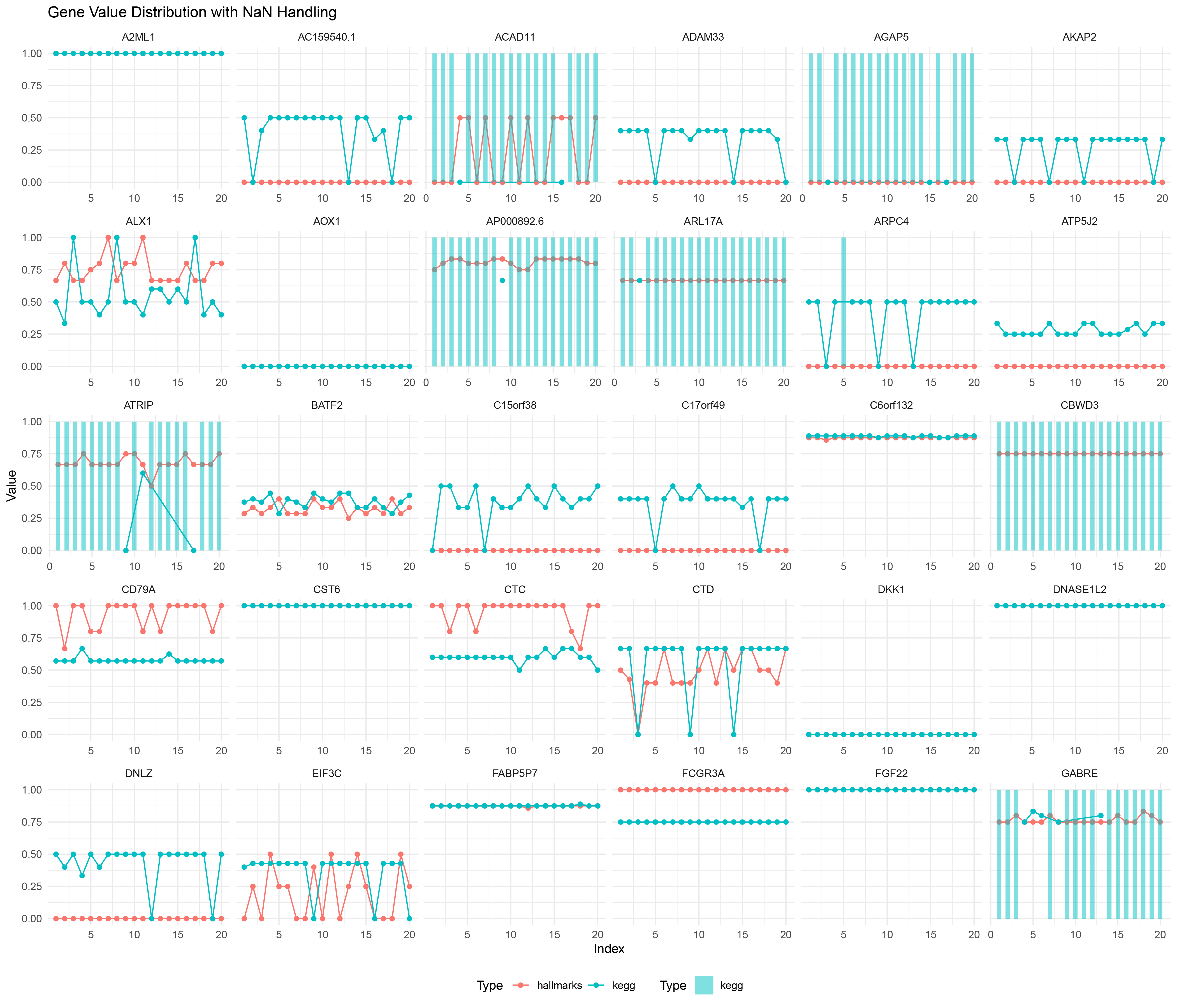

deseq2

16.5 outRst

outRst_positive_negative_ratio_list_data <- data.frame(
  Gene_Type = names(outRst_positive_negative_ratio_list),
  Value = unlist(outRst_positive_negative_ratio_list)
)

outRst_positive_negative_ratio_list_data <- outRst_positive_negative_ratio_list_data %>%
  mutate(Gene = sub("_.*", "", Gene_Type),
         Type = sub(".*_(.*)_.*", "\\1", Gene_Type),
         Index = as.numeric(sub(".*_", "", Gene_Type)))

head(outRst_positive_negative_ratio_list_data)


ggplot() +
  geom_line(data = outRst_positive_negative_ratio_list_data %>% filter(!is.na(Value)), 
            aes(x = Index, y = Value, color = Type, group = interaction(Gene, Type))) +
  geom_point(data = outRst_positive_negative_ratio_list_data %>% filter(!is.na(Value)), 
             aes(x = Index, y = Value, color = Type, group = interaction(Gene, Type))) +
  geom_bar(data = outRst_positive_negative_ratio_list_data %>% filter(is.na(Value)), 
           aes(x = Index, y = 1, fill = Type), stat = "identity", alpha = 0.5, width = 0.5) +
  scale_fill_manual(values = c("hallmarks" = "#F8766D", "kegg" = "#00BFC4")) + 
  facet_wrap(~ Gene, scales = "free_x") +
  labs(title = "Gene Value Distribution with NaN Handling",
       x = "Index",
       y = "Value") +
  theme_minimal() +
  theme(legend.position = "bottom")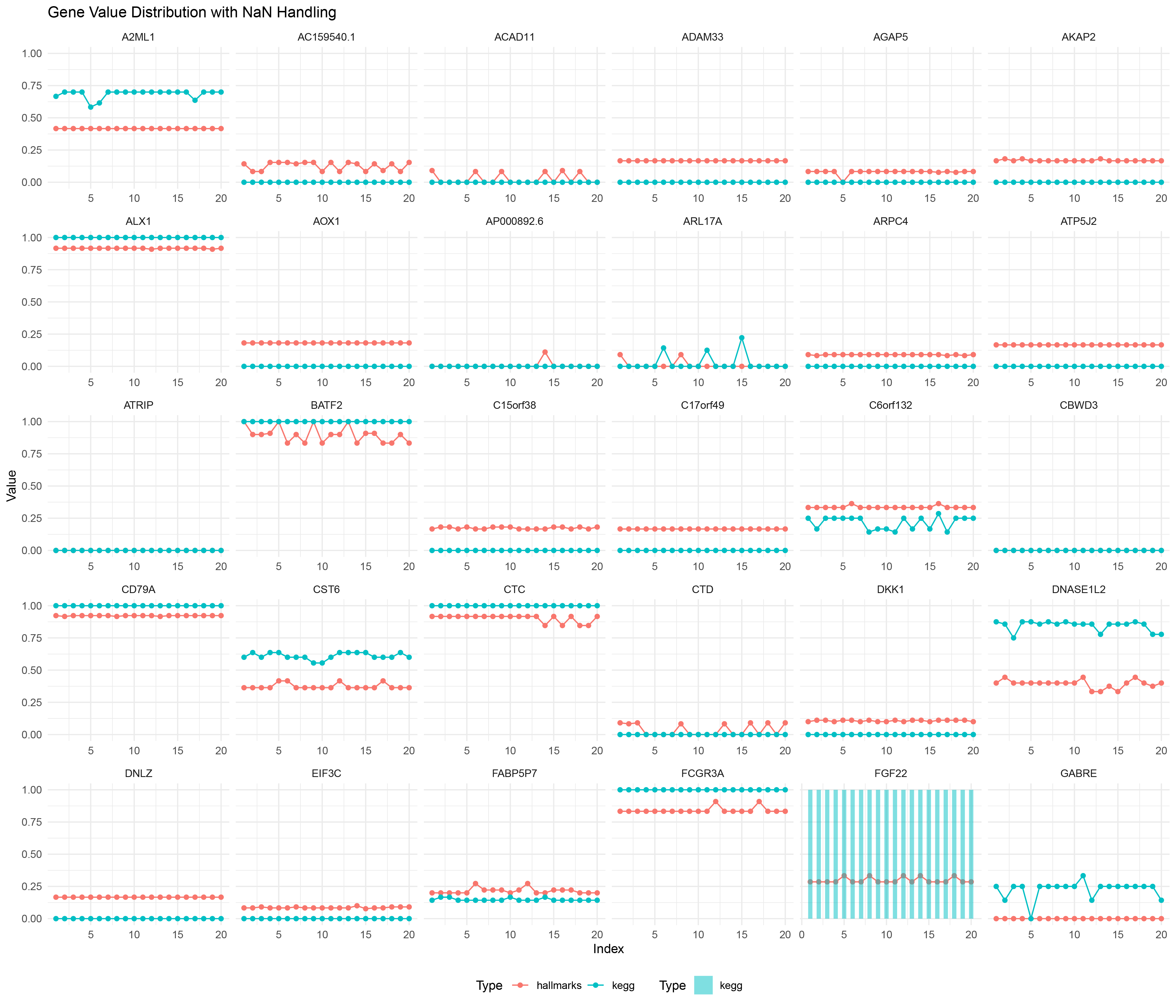

WRST

16.6 limma

limma_positive_negative_ratio_list_data <- data.frame(
  Gene_Type = names(limma_positive_negative_ratio_list),
  Value = unlist(limma_positive_negative_ratio_list)
)

limma_positive_negative_ratio_list_data <- limma_positive_negative_ratio_list_data %>%
  mutate(Gene = sub("_.*", "", Gene_Type),
         Type = sub(".*_(.*)_.*", "\\1", Gene_Type),
         Index = as.numeric(sub(".*_", "", Gene_Type)))

head(limma_positive_negative_ratio_list_data)

ggplot() +
  geom_line(data = limma_positive_negative_ratio_list_data %>% filter(!is.na(Value)), 
            aes(x = Index, y = Value, color = Type, group = interaction(Gene, Type))) +
  geom_point(data = limma_positive_negative_ratio_list_data %>% filter(!is.na(Value)), 
             aes(x = Index, y = Value, color = Type, group = interaction(Gene, Type))) +
  geom_bar(data = limma_positive_negative_ratio_list_data %>% filter(is.na(Value)), 
           aes(x = Index, y = 1, fill = Type), stat = "identity", alpha = 0.5, width = 0.5) +
  scale_fill_manual(values = c("hallmarks" = "#F8766D", "kegg" = "#00BFC4")) +  
  facet_wrap(~ Gene, scales = "free_x") +
  labs(title = "Gene Value Distribution with NaN Handling",
       x = "Index",
       y = "Value") +
  theme_minimal() +
  theme(legend.position = "bottom")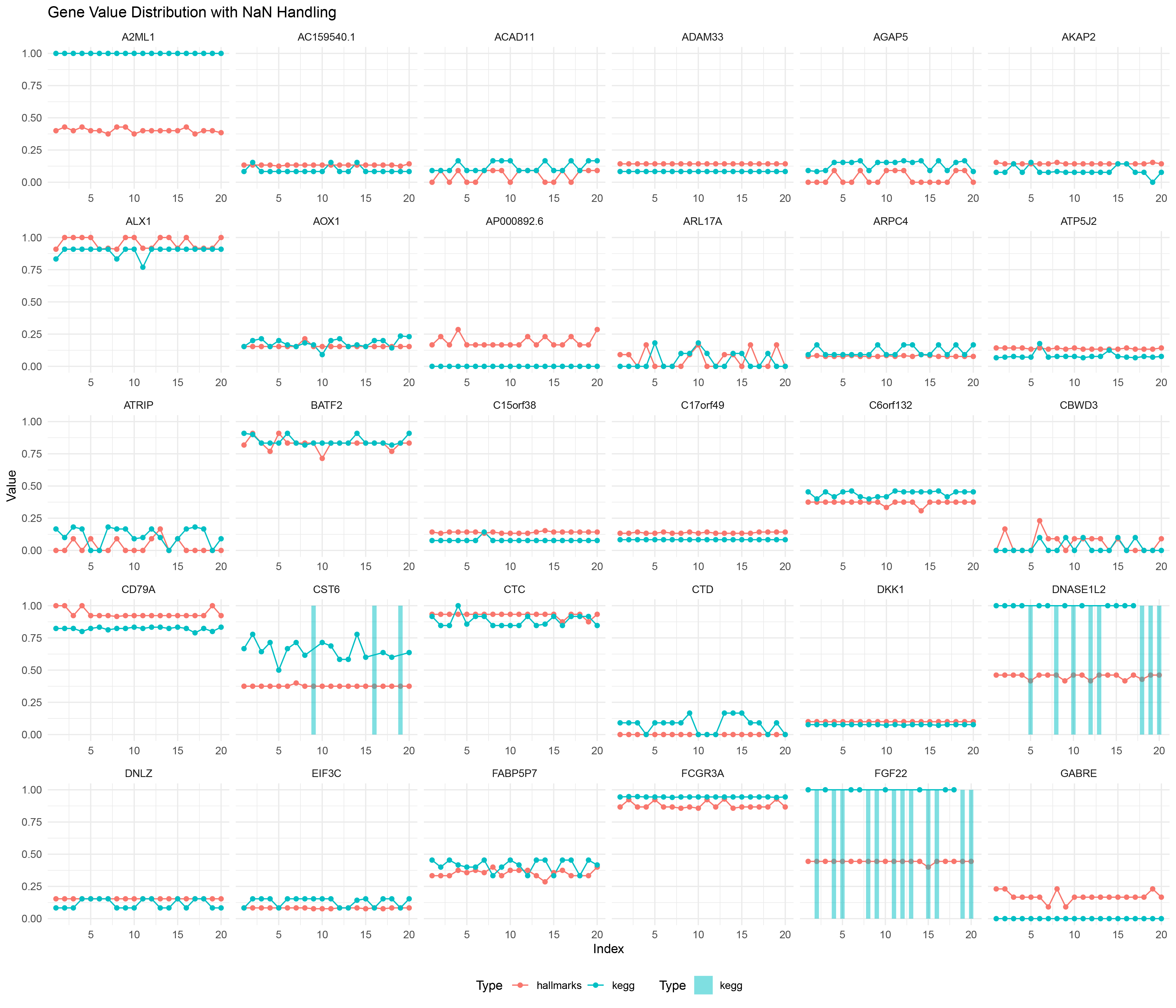

limma

16.7 edgeR

edgeR_positive_negative_ratio_list_data <- data.frame(
  Gene_Type = names(edgeR_positive_negative_ratio_list),
  Value = unlist(edgeR_positive_negative_ratio_list)
)

edgeR_positive_negative_ratio_list_data <- edgeR_positive_negative_ratio_list_data %>%
  mutate(Gene = sub("_.*", "", Gene_Type),
         Type = sub(".*_(.*)_.*", "\\1", Gene_Type),
         Index = as.numeric(sub(".*_", "", Gene_Type)))

head(edgeR_positive_negative_ratio_list_data)


ggplot() +
  geom_line(data = edgeR_positive_negative_ratio_list_data %>% filter(!is.na(Value)), 
            aes(x = Index, y = Value, color = Type, group = interaction(Gene, Type))) +
  geom_point(data = edgeR_positive_negative_ratio_list_data %>% filter(!is.na(Value)), 
             aes(x = Index, y = Value, color = Type, group = interaction(Gene, Type))) +
  geom_bar(data = edgeR_positive_negative_ratio_list_data %>% filter(is.na(Value)), 
           aes(x = Index, y = 1, fill = Type), stat = "identity", alpha = 0.5, width = 0.5) +
  scale_fill_manual(values = c("hallmarks" = "#F8766D", "kegg" = "#00BFC4")) +  
  facet_wrap(~ Gene, scales = "free_x") +
  labs(title = "Gene Value Distribution with NaN Handling",
       x = "Index",
       y = "Value") +
  theme_minimal() +
  theme(legend.position = "bottom")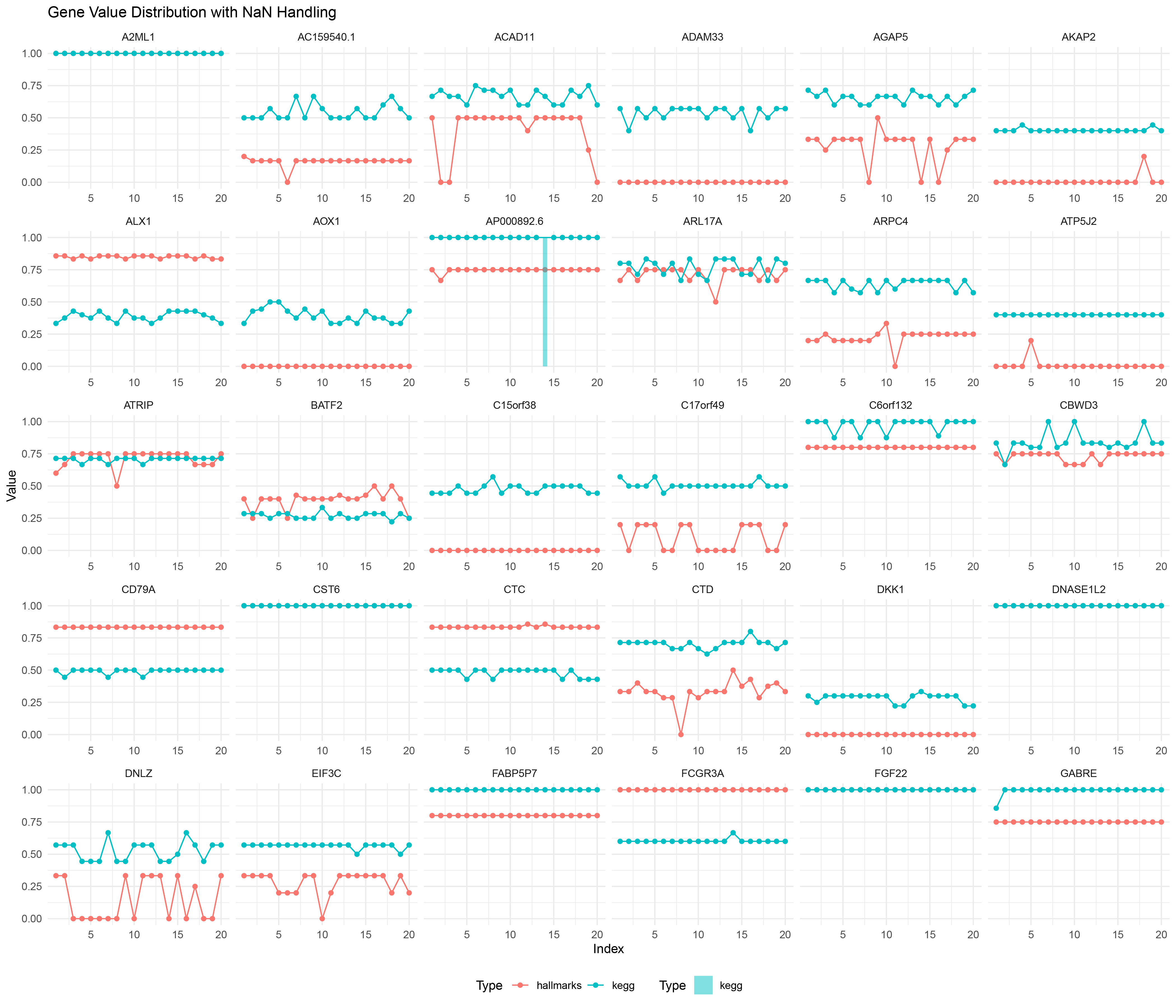

edgeR

16.8 hallmarks

# Add data source identifiers
deseq2_positive_negative_ratio_list_data1 <- deseq2_positive_negative_ratio_list_data %>% mutate(Source = "deseq2")
edgeR_positive_negative_ratio_list_data1 <- edgeR_positive_negative_ratio_list_data %>% mutate(Source = "edgeR")
TransPropy2_positive_negative_ratio_list_data1 <- TransPropy2_positive_negative_ratio_list_data %>% mutate(Source = "TransPropy2")
outRst_positive_negative_ratio_list_data1 <- outRst_positive_negative_ratio_list_data %>% mutate(Source = "outRst")
limma_positive_negative_ratio_list_data1 <- limma_positive_negative_ratio_list_data %>% mutate(Source = "limma")

# Merge all data frames
all_data1 <- bind_rows(
  deseq2_positive_negative_ratio_list_data1,
  edgeR_positive_negative_ratio_list_data1,
  TransPropy2_positive_negative_ratio_list_data1,
  outRst_positive_negative_ratio_list_data1,
  limma_positive_negative_ratio_list_data1
)

# Convert the Gene column to a factor and specify the order of factor levels
all_data1$Gene <- factor(all_data1$Gene, levels = unique(all_data1$Gene))


colors <- c("deseq2" = "#3273c1", "edgeR" = "#2b8f9a", "TransPropy2" = "#6e4ab4", 
            "outRst" = "#48884d", "limma" = "#a8a74e")

# Handle NaN values, calculate segment heights
nan_data <- all_data1 %>%
  filter(is.na(Value)) %>%
  group_by(Gene, Type) %>%
  mutate(n_sources = n_distinct(Source), 
         height = 1 / n_sources) %>%
  ungroup()

nan_data$Gene <- factor(nan_data$Gene, levels = unique(all_data1$Gene))


print(nan_data)


ggplot() +
  geom_line(data = all_data1 %>% filter(Type == "hallmarks", !is.na(Value)), 
            aes(x = Gene, y = Value, color = Source, group = interaction(Gene, Source)), size = 1) +
  geom_point(data = all_data1 %>% filter(Type == "hallmarks", !is.na(Value)), 
             aes(x = Gene, y = Value, color = Source, group = interaction(Gene, Source)), size = 3) +
  geom_smooth(data = all_data1 %>% filter(Type == "hallmarks" & !is.na(Value)), 
              aes(x = as.numeric(Gene), y = Value, color = Source, fill = Source), method = "lm", se = TRUE, alpha = 0.2) +
  geom_segment(data = nan_data %>% filter(Type == "hallmarks"), 
               aes(x = Gene, xend = Gene, y = 0, yend = height, color = Source), size = 1, alpha = 0.4) +
  scale_color_manual(values = colors) +  
  scale_fill_manual(values = colors) +  
  scale_x_discrete(limits = levels(all_data1$Gene)) + # Ensure the X-axis order is consistent with the factor order
  labs(title = "Hallmarks Gene Value Distribution",
       x = "Gene",
       y = "Value") +
  ylim(0, 1) +  
  theme_minimal() +
  theme(axis.text.x = element_text(angle = 90, hjust = 1), legend.position = "bottom")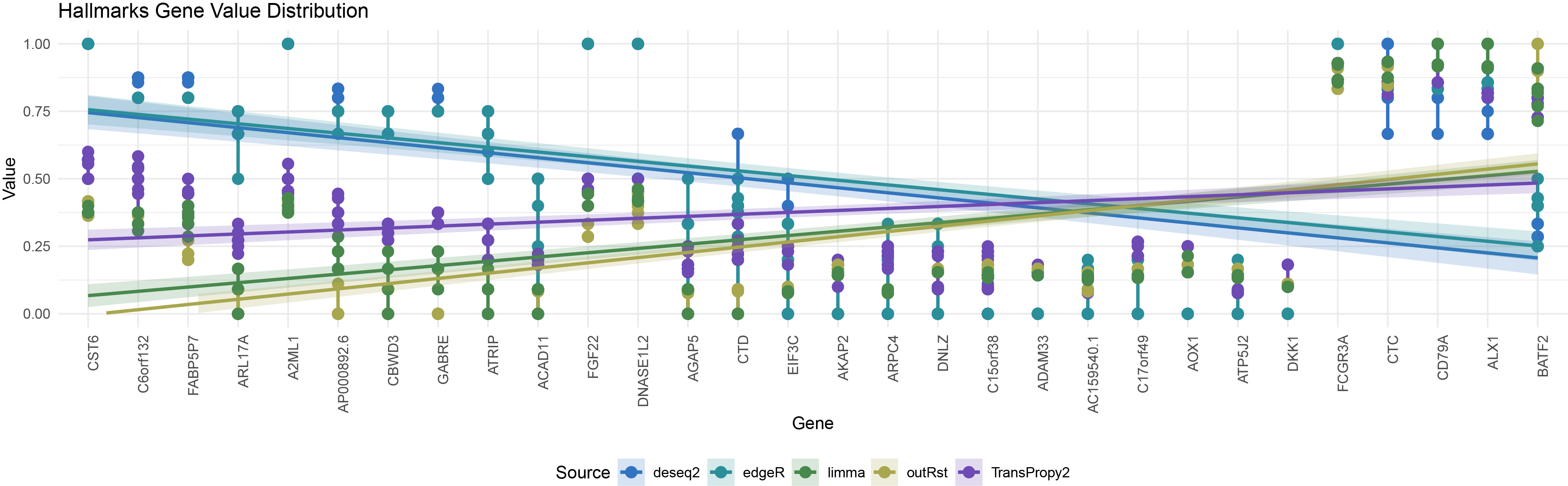

hallmarks_all

16.9 kegg

deseq2_positive_negative_ratio_list_data1 <- deseq2_positive_negative_ratio_list_data %>% mutate(Source = "deseq2")
edgeR_positive_negative_ratio_list_data1 <- edgeR_positive_negative_ratio_list_data %>% mutate(Source = "edgeR")
TransPropy2_positive_negative_ratio_list_data1 <- TransPropy2_positive_negative_ratio_list_data %>% mutate(Source = "TransPropy2")
outRst_positive_negative_ratio_list_data1 <- outRst_positive_negative_ratio_list_data %>% mutate(Source = "outRst")
limma_positive_negative_ratio_list_data1 <- limma_positive_negative_ratio_list_data %>% mutate(Source = "limma")


all_data1 <- bind_rows(
  deseq2_positive_negative_ratio_list_data1,
  edgeR_positive_negative_ratio_list_data1,
  TransPropy2_positive_negative_ratio_list_data1,
  outRst_positive_negative_ratio_list_data1,
  limma_positive_negative_ratio_list_data1
)


all_data1$Gene <- factor(all_data1$Gene, levels = unique(all_data1$Gene))

colors <- c("deseq2" = "#3273c1", "edgeR" = "#2b8f9a", "TransPropy2" = "#6e4ab4", 
            "outRst" = "#48884d", "limma" = "#a8a74e")


nan_data <- all_data1 %>%
  filter(is.na(Value)) %>%
  group_by(Gene, Type) %>%
  mutate(n_sources = n_distinct(Source), 
         height = 1 / n_sources) %>%
  ungroup() %>%
  arrange(Gene, Type, Source) %>%
  group_by(Gene) %>%
  mutate(cumulative_height = cumsum(ifelse(duplicated(Source), 0, height))) %>%
  ungroup() %>%
  mutate(y_start = cumulative_height - height, 
         y_end = cumulative_height)

nan_data$Gene <- factor(nan_data$Gene, levels = unique(all_data1$Gene))


print(nan_data)


ggplot() +
  geom_segment(data = nan_data %>% filter(Type == "kegg"), 
               aes(x = as.numeric(Gene), xend = as.numeric(Gene), y = y_start, yend = y_end, color = Source), 
               size = 7, alpha = 0.1) +
  geom_smooth(data = all_data1 %>% filter(Type == "kegg" & !is.na(Value)), 
              aes(x = as.numeric(Gene), y = Value, color = Source, fill = Source), method = "lm", se = TRUE, alpha = 0.2) +
  geom_line(data = all_data1 %>% filter(Type == "kegg" & !is.na(Value)), 
            aes(x = as.numeric(Gene), y = Value, color = Source, group = interaction(Gene, Source)), 
            size = 1) +
  geom_point(data = all_data1 %>% filter(Type == "kegg" & !is.na(Value)), 
             aes(x = as.numeric(Gene), y = Value, color = Source, group = interaction(Gene, Source)), 
             size = 3) +
  scale_color_manual(values = colors) +  
  scale_fill_manual(values = colors) + 
  scale_x_continuous(breaks = 1:length(levels(all_data1$Gene)), labels = levels(all_data1$Gene)) +  
  labs(title = "Kegg Gene Value Distribution",
       x = "Gene",
       y = "Value") +
  ylim(0, 1) +  
  theme_minimal() +
  theme(axis.text.x = element_text(angle = 90, hjust = 1), legend.position = "bottom")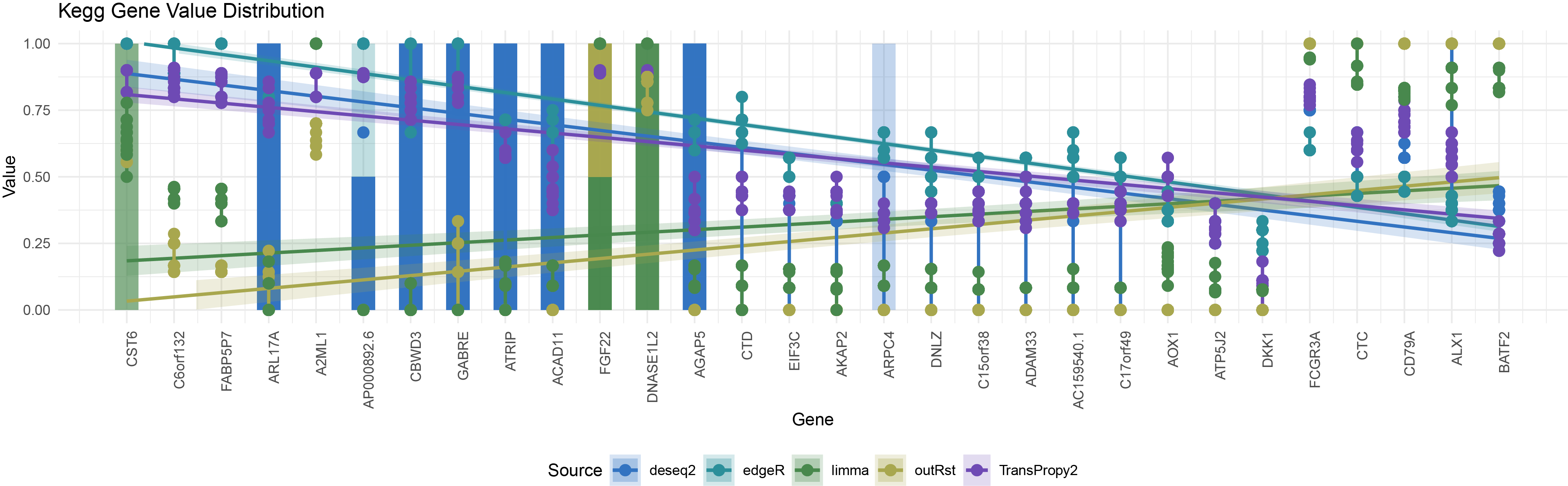

kegg_all