10 Comparison of TransPropy with Other Tool Packages Using Percentage Stacked Line Bar Chart
10.1 library
library(readr)
library(TransProR)
library(dplyr)
library(rlang)
library(linkET)
library(funkyheatmap)
library(tidyverse)
library(RColorBrewer)
library(ggalluvial)
library(tidyr)
library(tibble)
10.2 data
data = tribble(
  ~Methods,  ~DownRatio,  ~UpRatio,
  "deseq2",  666,  899,
  "edgeR",  685,  788,
  "limma", 757, 1022,
  "Rank-Sum Test",  579,  1089,
  "TransPropy",  711,  726
)

data %>%
  mutate(id = 1:n()) %>%
  pivot_longer(-c(id, Methods), names_to = "shade", values_to = "value") -> df

pal = c('#909231', '#f4bf5f')
10.3 All Percentage Stacked Line Bar Chart
df %>%
  mutate(prop = round(value/sum(value)*100, 2), .by = Methods) %>%
  ggplot(aes(x=id, y=prop, fill=shade)) +
  geom_stratum(aes(stratum=shade), color=NA, width = 0.65) +
  geom_flow(aes(alluvium=shade), knot.pos = 0.25, width = 0.65, alpha=0.5) +
  geom_alluvium(aes(alluvium=shade),
                knot.pos = 0.25, color="#f4e2de", width=0.65, linewidth=0.5, fill=NA, alpha=1) +
  scale_fill_manual(values = pal) +
  scale_x_continuous(expand = c(0, 0), breaks = 1:5, labels = data$Methods, name = NULL) +
  scale_y_continuous(expand = c(0, 0),
                      # limits = c(0, 10000),
                      name = NULL) +
  geom_hline(yintercept = c(50),
              linewidth = 3,
              color = 'white',
              lty = 'dashed',
              alpha = 0.5)+
  geom_hline(yintercept = c(25,75),
              linewidth = 1.5,
              color = 'white',
              lty = 'dashed',
              alpha = 0.5)+
  labs(title = "Percentage Stacked Line Bar Chart",
        subtitle = "Comparison of Five Feature Extraction Methods. \nProportion Comparison of Negatively and Positively Correlated Feature Genes. ") +
  theme_minimal() +
  theme(plot.background = element_rect(fill='white', color='white'),
        panel.grid = element_blank())
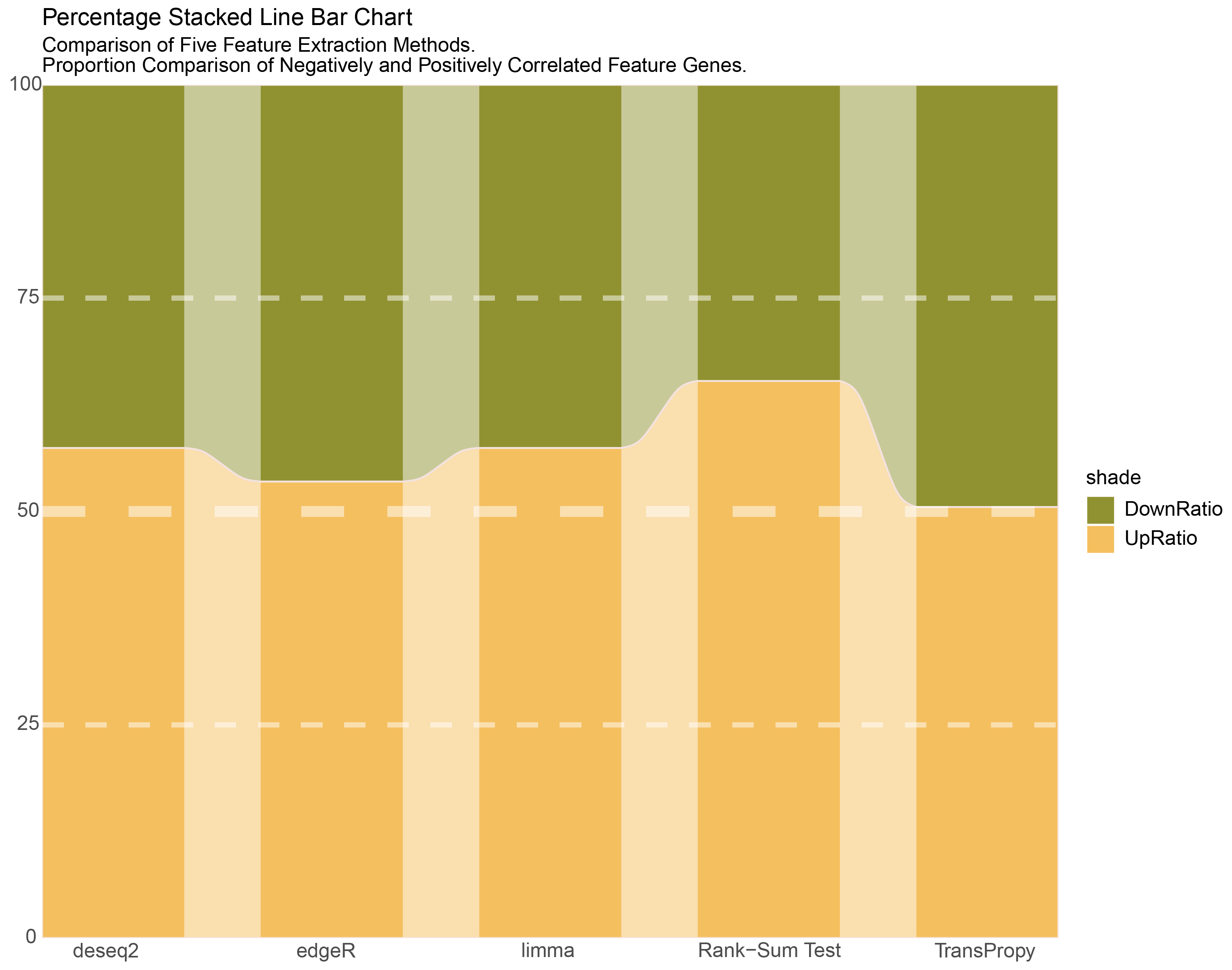
All Percentage Stacked Line Bar Chart.png
10.4 Separate Percentage Stacked Line Bar Chart
# Create the transformed data frame with all Down columns first and Up columns at the end
data <- tribble(
  ~Methods,    ~Down_A2ML1, ~Down_AC159540.1, ~Down_ACAD11, ~Down_ADAM33, ~Down_AGAP5,
  ~Down_AKAP2, ~Down_ALOXE3, ~Down_ALX1, ~Down_ANKRD35, ~Down_AOX1,
  ~Down_AP000892.6, ~Down_ARL17A, ~Down_ARPC4.TTLL3, ~Down_ATP5J2.PTCD1, ~Down_ATRIP, ~Down_BATF2, ~Down_C15orf38.AP3S2, ~Down_C17orf49, ~Down_C6orf132,
  ~Down_CBWD3, ~Down_CD79A, ~Down_CFD, ~Down_CST6, ~Down_CTC.231O11.1,
  ~Down_CTD.2231E14.8, ~Down_DKK1, ~Down_DNASE1L2, ~Down_DNLZ, ~Down_EIF3C,
  ~Down_FABP5P7, ~Down_FCGR3A, ~Down_FGF22, ~Down_GABRE,
  ~Up_A2ML1, ~Up_AC159540.1, ~Up_ACAD11, ~Up_ADAM33, ~Up_AGAP5,
  ~Up_AKAP2, ~Up_ALOXE3, ~Up_ALX1, ~Up_ANKRD35, ~Up_AOX1,
  ~Up_AP000892.6, ~Up_ARL17A, ~Up_ARPC4.TTLL3, ~Up_ATP5J2.PTCD1, ~Up_ATRIP, ~Up_BATF2, ~Up_C15orf38.AP3S2, ~Up_C17orf49, ~Up_C6orf132,
  ~Up_CBWD3, ~Up_CD79A, ~Up_CFD, ~Up_CST6, ~Up_CTC.231O11.1,
  ~Up_CTD.2231E14.8, ~Up_DKK1, ~Up_DNASE1L2, ~Up_DNLZ, ~Up_EIF3C,
  ~Up_FABP5P7, ~Up_FCGR3A, ~Up_FGF22, ~Up_GABRE,
  "deseq2",        194,           877,           852,          880,       849,
  900,           292,          621,           619,       767,
  737,           816,          859,          804,       837,
  1143,           904,          884,           710,       805,
  586,            453,          290,           548,       865,
  104,            40,           881,           882,       685,
  491,            28,           775,
  978,            666,         1028,         615,        912,
  583,          1035,         876,         1190,        513,
  1232,          1224,          748,          504,       1169,
  889,           627,          653,         1212,       1243,
  882,          1133,         1075,          942,        927,
  131,           976,          673,          739,       1188,
  938,           923,         1255,
  "edgeR",         175,           943,           911,          938,       910,
  956,           282,          540,           648,       791,
  777,           875,          920,          837,       899,
  958,           975,          946,           752,       863,
  514,            464,          284,           478,       924,
  106,             35,          950,           954,       730,
  428,             25,          826,
  810,            564,          864,          528,        774,
  501,           861,          930,          984,        446,
  1022,          1015,          634,          438,        981,
  967,           541,          561,         1000,       1031,
  961,           935,          885,         1012,        803,
  122,           810,          585,          637,        988,
  1024,           765,         1036,
  "limma",         343,          1031,           934,         1014,       972,
  969,           389,          744,           605,       884,
  673,           838,         1025,          886,       927,
  1257,           987,          998,           664,       806,
  676,            489,          379,           669,      1033,
  346,            253,         1049,          954,       610,
  551,            228,          735,
  1070,            804,         1130,          735,       1035,
  674,          1129,         1104,         1307,        610,
  1383,          1349,          895,          598,       1278,
  1048,           744,          790,         1330,       1368,
  1101,          1290,         1145,         1130,       1063,
  167,          1047,          810,          892,       1290,
  1041,          1002,         1380,
  "Rank-Sum Test", 183,           758,           681,          742,       695,
  745,           218,          787,           393,       683,
  454,           600,          732,          687,       665,
  1404,           750,          747,           443,       576,
  728,            288,          216,           700,       739,
  274,            116,          758,           747,       396,
  370,            100,          512,
  1288,            863,         1241,          791,      1128,
  734,          1345,          773,         1518,        659,
  1575,          1537,          970,          652,       1415,
  727,           801,          848,         1539,       1579,
  767,          1480,         1363,         1130,       1138,
  198,          1264,          865,          944,       1512,
  805,          1217,         1596,
  "TransPropy",    388,           969,           942,          954,       957,
  918,           502,          437,           782,       780,
  820,           930,          973,          776,       957,
  676,           933,          912,           844,       905,
  397,            646,          490,           409,      1000,
  177,            242,          997,          981,       797,
  370,            219,          863,
  655,            548,          695,          529,       645,
  502,           699,         1083,           822,       460,
  851,            817,          602,          432,       737,
  1092,           514,          539,           834,       850,
  1083,            755,          715,         1127,        612,
  143,           666,          545,          553,        817,
  1030,            621,          877
)
data %>%
mutate(id = 1:n()) %>%
pivot_longer(-c(id, Methods), names_to = "shade", values_to = "value") -> df
# Define the color palette
pal <- rev(c('#f5b7bb', '#f5b090','#f5b86d', '#eec040','#ddb918', '#cab600','#a2ac07', '#5d9000','#007308', '#007201','#005c25', '#00453a'))
# Generate 33 gradient colors from the first two colors
gradient1 <- rev(colorRampPalette(pal[1:6])(33))
# Generate 33 gradient colors from the last two colors
gradient2 <- rev(colorRampPalette(pal[7:12])(33))
# Combine the gradients
combined_gradient <- c(gradient1, gradient2)
# Print the combined gradient
print(combined_gradient)df %>%
mutate(prop = round(value/sum(value)*100, 2), .by = Methods) %>%
ggplot(aes(x=id, y=prop, fill=shade)) +
geom_stratum(aes(stratum=shade), color=NA, width = 0.65) +
geom_flow(aes(alluvium=shade), knot.pos = 0.25, width = 0.65, alpha=0.5) +
geom_alluvium(aes(alluvium=shade),
knot.pos = 0.25, color="#e9dfd3", width=0.65, linewidth=0.2, fill=NA, alpha=1) +
scale_fill_manual(values = combined_gradient) +
scale_x_continuous(expand = c(0, 0), breaks = 1:5, labels = data$Methods, name = NULL) +
scale_y_continuous(expand = c(0, 0),
# limits = c(0, 10000),
name = NULL) +
geom_hline(yintercept = c(50),
linewidth = 3,
color = 'white',
lty = 'dashed',
alpha = 0.5)+
geom_hline(yintercept = c(25,75),
linewidth = 1.5,
color = 'white',
lty = 'dashed',
alpha = 0.5)+
labs(title = "Percentage Stacked Line Bar Chart",
subtitle = "Comparison of Five Feature Extraction Methods. \nProportion Comparison of Negatively and Positively Correlated Feature Genes. ") +
theme_minimal() +
theme(plot.background = element_rect(fill='white', color='white'),
panel.grid = element_blank())+
guides(fill = guide_legend(ncol = 2)) # Set the number of legend columns to 2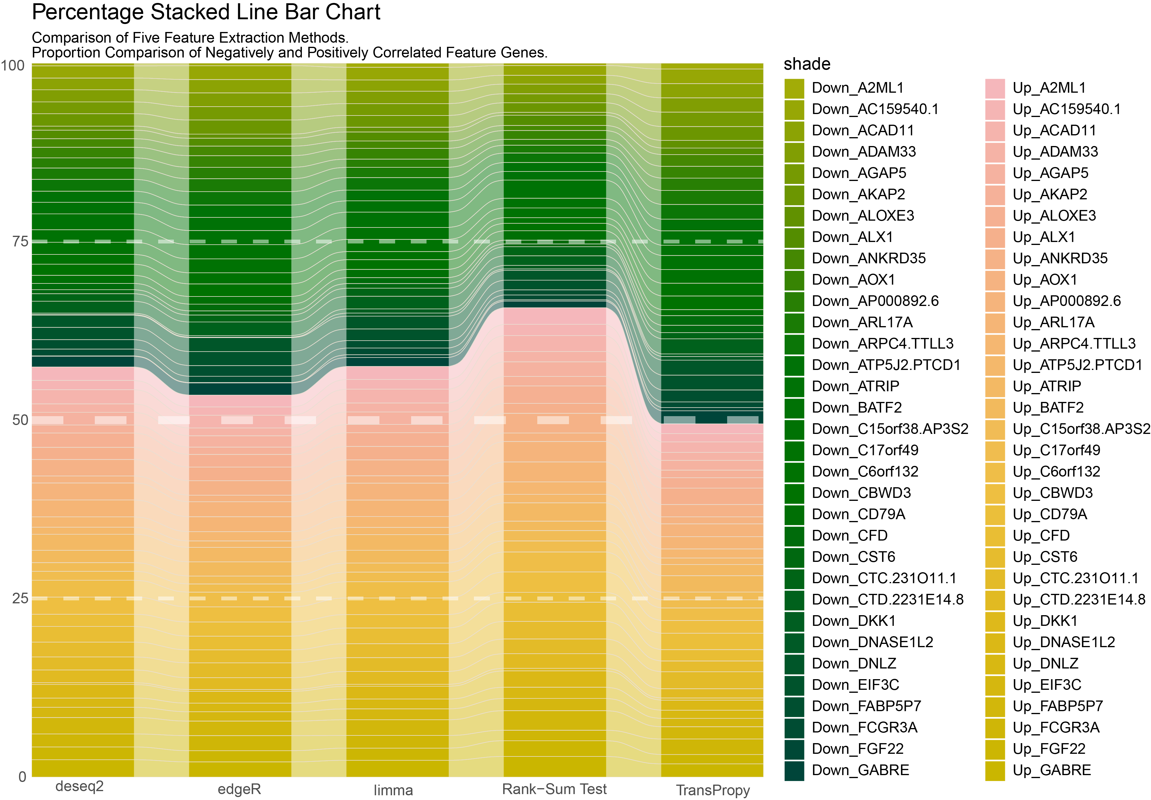
Separate Percentage Stacked Line Bar Chart
10.5 Methods
- Based on the results of Chapter 9, further calculate the sum of genes with an absolute value of positive or negative correlation greater than 0.5 for each intersection gene in each method, and create an All Percentage Stacked Line Bar Chart.
- Based on the results of Chapter 9, further calculate the number of genes with an absolute value of positive or negative correlation greater than 0.5 for each intersection gene in each method, and create separate Percentage Stacked Line Bar Charts for each method.
10.6 Discussion
DownRatio > UpRatio
DownRatio = UpRatio = 0.5 (BEST)
DownRatio > UpRatio